'%3e%3cpath id='Path_78' data-name='Path 78' d='M1231.387%2c253.519c-3.705-3.621-10.085-3.474-17.475-3.3-1.694.039-3.446.08-5.252.08-2.256%2c0-4.42-.086-6.514-.168-7-.274-13.045-.513-16.639%2c2.941-2.412%2c2.319-3.585%2c6.212-3.585%2c11.9%2c0%2c5.393%2c1.15%2c9.139%2c3.518%2c11.452%2c3.705%2c3.621%2c10.086%2c3.474%2c17.474%2c3.3%2c1.694-.039%2c3.446-.08%2c5.253-.08%2c2.256%2c0%2c4.42.085%2c6.514.168%2c1.852.073%2c3.636.143%2c5.327.143%2c4.7%2c0%2c8.668-.544%2c11.311-3.085%2c2.413-2.319%2c3.585-6.211%2c3.585-11.9C1234.9%2c259.577%2c1233.755%2c255.832%2c1231.387%2c253.519Zm-.674%2c22.719c-3.325%2c3.2-8.918%2c2.975-16%2c2.7-2.1-.082-4.275-.168-6.548-.168-1.817%2c0-3.574.041-5.273.08-7.487.173-13.4.31-16.842-3.052-2.19-2.14-3.254-5.68-3.254-10.825%2c0-5.437%2c1.085-9.122%2c3.316-11.268%2c3.325-3.2%2c8.919-2.975%2c16-2.7%2c2.1.083%2c4.276.168%2c6.549.168%2c1.817%2c0%2c3.574-.04%2c5.273-.08%2c7.487-.173%2c13.4-.31%2c16.842%2c3.053%2c2.19%2c2.139%2c3.254%2c5.679%2c3.254%2c10.824C1234.029%2c270.407%2c1232.944%2c274.093%2c1230.713%2c276.238Z' transform='translate(-1181.922 -239.039)'%3e%3c/path%3e%3cpath id='Path_79' data-name='Path 79' d='M1229.229%2c246.046c-3.479-2.38-8.5-3.489-15.809-3.489-11.45%2c0-22.628%2c1.422-22.628%2c18.425%2c0%2c7.138%2c2.069%2c12.024%2c6.326%2c14.937%2c3.479%2c2.381%2c8.5%2c3.489%2c15.81%2c3.489%2c11.45%2c0%2c22.629-1.422%2c22.629-18.426C1235.556%2c253.844%2c1233.486%2c248.959%2c1229.229%2c246.046Zm-16.3%2c32.487c-11.042%2c0-21.26-2.127-21.26-17.551%2c0-16.207%2c10.289-17.549%2c21.752-17.549%2c11.042%2c0%2c21.26%2c2.127%2c21.26%2c17.549C1234.68%2c277.19%2c1224.39%2c278.533%2c1212.927%2c278.533Z' transform='translate(-1186.682 -235.052)'%3e%3c/path%3e%3cpath id='Path_80' data-name='Path 80' d='M1218.178%2c234.457c-11.25%2c0-18.52%2c8.705-18.52%2c22.178%2c0%2c13.266%2c7.245%2c22.179%2c18.027%2c22.179%2c11.25%2c0%2c18.52-8.705%2c18.52-22.179C1236.206%2c243.37%2c1228.961%2c234.457%2c1218.178%2c234.457Zm-.492%2c43.481c-10.259%2c0-17.151-8.561-17.151-21.3%2c0-12.941%2c6.925-21.3%2c17.643-21.3%2c10.259%2c0%2c17.151%2c8.561%2c17.151%2c21.3C1235.33%2c269.576%2c1228.4%2c277.938%2c1217.686%2c277.938Z' transform='translate(-1191.441 -230.705)'%3e%3c/path%3e%3cpath id='Path_81' data-name='Path 81' d='M1222.938%2c226.358c-3.9%2c0-7.578%2c2.983-10.368%2c8.4a39.516%2c39.516%2c0%2c0%2c0-4.042%2c17.531c0%2c10.6%2c4.957%2c25.932%2c13.918%2c25.932%2c3.9%2c0%2c7.578-2.983%2c10.368-8.4a39.509%2c39.509%2c0%2c0%2c0%2c4.043-17.531C1236.857%2c241.69%2c1231.9%2c226.358%2c1222.938%2c226.358Zm-.492%2c50.987c-3.646%2c0-7.03-2.988-9.527-8.412a41.8%2c41.8%2c0%2c0%2c1-3.515-16.644c0-11.827%2c5.788-25.055%2c13.534-25.055%2c3.646%2c0%2c7.03%2c2.988%2c9.528%2c8.413a41.8%2c41.8%2c0%2c0%2c1%2c3.515%2c16.643C1235.981%2c264.116%2c1230.192%2c277.344%2c1222.446%2c277.344Z' transform='translate(-1196.201 -226.358)'%3e%3c/path%3e%3c/g%3e%3c/svg%3e)
'%3e%3cg transform='translate(1235.906 232.606)'%3e%3cpath d='M1343.067%2c255.169h1.652l-.012%2c2.917c.365-1.823%2c2.735-3.282%2c7.11-3.282%2c5.47%2c0%2c7.657%2c2.552%2c7.657%2c8.022V273.4h-1.823v-9.48c0-5.834-1.641-7.293-6.381-7.293-5.47%2c0-6.381%2c2.443-6.381%2c7.293v9.48h-1.823Z' transform='translate(-1343.067 -251.523)'%3e%3c/path%3e%3cpath d='M1410%2c265.744v-2.917c0-5.287%2c1.823-8.022%2c8.386-8.022s8.386%2c2.735%2c8.386%2c8.022v2.917c0%2c5.469-1.823%2c8.022-8.386%2c8.022S1410%2c271.213%2c1410%2c265.744Zm14.95%2c0v-2.917c0-4.193-.839-6.2-6.563-6.2s-6.563%2c2.005-6.563%2c6.2v2.917c0%2c4.193.839%2c6.2%2c6.563%2c6.2S1424.953%2c269.937%2c1424.953%2c265.744Z' transform='translate(-1387.58 -251.523)'%3e%3c/path%3e%3cpath d='M1485.684%2c274.489c-5.47%2c0-7.657-2.553-7.657-8.022V255.893h1.823v9.48c0%2c5.834%2c1.641%2c7.293%2c6.381%2c7.293%2c5.469%2c0%2c6.381-2.37%2c6.381-7.293v-9.48h1.823v18.231H1492.8l-.006-2.917C1492.43%2c273.031%2c1490.06%2c274.489%2c1485.684%2c274.489Z' transform='translate(-1432.815 -252.247)'%3e%3c/path%3e%3cpath d='M1612.443%2c265.744v-2.917c0-5.287%2c1.823-8.022%2c8.386-8.022s8.386%2c2.735%2c8.386%2c8.022v2.917c0%2c5.469-1.823%2c8.022-8.386%2c8.022S1612.443%2c271.213%2c1612.443%2c265.744Zm14.95%2c0v-2.917c0-4.193-.839-6.2-6.563-6.2s-6.563%2c2.005-6.563%2c6.2v2.917c0%2c4.193.839%2c6.2%2c6.563%2c6.2S1627.393%2c269.937%2c1627.393%2c265.744Z' transform='translate(-1522.202 -251.523)'%3e%3c/path%3e%3cpath d='M1691.406%2c266.887h-3.646c-5.287%2c0-7.293-2.005-7.293-7.293V245.009h1.823v3.646h9.116v1.823h-9.116v9.115c0%2c4.74%2c1.823%2c5.469%2c5.47%2c5.469h3.646Z' transform='translate(-1567.438 -245.009)'%3e%3c/path%3e%3cpath d='M1553.711%2c263.374c-4.3-.511-6.381-1.276-6.381-3.647%2c0-2.188%2c1.385-3.1%2c6.381-3.1%2c4.708%2c0%2c6.088.785%2c6.334%2c3.094h1.849c-.211-3.154-2.32-4.917-8.184-4.917-5.944%2c0-8.2%2c1.823-8.2%2c4.922%2c0%2c3.464%2c1.75%2c4.776%2c8.2%2c5.469%2c4.558.547%2c6.746%2c1.276%2c6.746%2c3.646%2c0%2c2.188-1.458%2c3.1-6.746%2c3.1-4.726%2c0-6.1-.82-6.337-3.129h-1.849c.2%2c3.175%2c2.3%2c4.952%2c8.186%2c4.952%2c6.2%2c0%2c8.569-1.823%2c8.569-4.923C1562.28%2c265.379%2c1560.457%2c264.1%2c1553.711%2c263.374Z' transform='translate(-1477.69 -251.523)'%3e%3c/path%3e%3c/g%3e%3cg transform='translate(1181.922 226.358)'%3e%3cpath d='M1217.687%2c252.541c-2.679-2.618-7.292-2.512-12.635-2.387-1.225.029-2.491.058-3.8.058-1.631%2c0-3.2-.062-4.71-.122-5.061-.2-9.432-.371-12.031%2c2.127-1.744%2c1.677-2.592%2c4.491-2.592%2c8.6%2c0%2c3.9.832%2c6.608%2c2.544%2c8.28%2c2.679%2c2.618%2c7.292%2c2.512%2c12.635%2c2.387%2c1.225-.029%2c2.492-.058%2c3.8-.058%2c1.631%2c0%2c3.2.062%2c4.71.122%2c1.339.053%2c2.629.1%2c3.852.1%2c3.4%2c0%2c6.268-.393%2c8.179-2.23%2c1.744-1.677%2c2.592-4.491%2c2.592-8.6C1220.231%2c256.921%2c1219.4%2c254.213%2c1217.687%2c252.541Zm-.487%2c16.427c-2.4%2c2.311-6.448%2c2.151-11.567%2c1.95-1.52-.06-3.091-.122-4.734-.122-1.314%2c0-2.584.029-3.813.058-5.413.125-9.688.224-12.177-2.207-1.583-1.547-2.353-4.107-2.353-7.827%2c0-3.931.784-6.6%2c2.4-8.147%2c2.4-2.311%2c6.449-2.151%2c11.566-1.95%2c1.52.06%2c3.092.122%2c4.735.122%2c1.313%2c0%2c2.584-.029%2c3.813-.058%2c5.413-.125%2c9.689-.224%2c12.178%2c2.207%2c1.583%2c1.547%2c2.353%2c4.106%2c2.353%2c7.826C1219.6%2c264.751%2c1218.813%2c267.416%2c1217.2%2c268.967Z' transform='translate(-1181.922 -242.071)'%3e%3c/path%3e%3cpath d='M1218.583%2c245.08c-2.516-1.721-6.148-2.523-11.431-2.523-8.279%2c0-16.361%2c1.028-16.361%2c13.322%2c0%2c5.161%2c1.5%2c8.694%2c4.574%2c10.8%2c2.516%2c1.721%2c6.148%2c2.523%2c11.431%2c2.523%2c8.279%2c0%2c16.361-1.028%2c16.361-13.323C1223.158%2c250.718%2c1221.661%2c247.186%2c1218.583%2c245.08ZM1206.8%2c268.569c-7.984%2c0-15.372-1.538-15.372-12.69%2c0-11.718%2c7.44-12.689%2c15.728-12.689%2c7.984%2c0%2c15.372%2c1.538%2c15.372%2c12.689C1222.524%2c267.6%2c1215.085%2c268.569%2c1206.8%2c268.569Z' transform='translate(-1187.82 -237.13)'%3e%3c/path%3e%3cpath d='M1213.049%2c234.457c-8.134%2c0-13.39%2c6.294-13.39%2c16.035%2c0%2c9.592%2c5.238%2c16.036%2c13.035%2c16.036%2c8.134%2c0%2c13.39-6.294%2c13.39-16.036C1226.084%2c240.9%2c1220.846%2c234.457%2c1213.049%2c234.457Zm-.356%2c31.438c-7.418%2c0-12.4-6.19-12.4-15.4%2c0-9.357%2c5.007-15.4%2c12.757-15.4%2c7.417%2c0%2c12.4%2c6.19%2c12.4%2c15.4C1225.45%2c259.849%2c1220.443%2c265.9%2c1212.694%2c265.9Z' transform='translate(-1193.717 -231.744)'%3e%3c/path%3e%3cpath d='M1218.947%2c226.358c-2.817%2c0-5.479%2c2.157-7.5%2c6.073a28.572%2c28.572%2c0%2c0%2c0-2.922%2c12.675c0%2c7.663%2c3.584%2c18.75%2c10.063%2c18.75%2c2.817%2c0%2c5.479-2.157%2c7.5-6.074a28.567%2c28.567%2c0%2c0%2c0%2c2.923-12.676C1229.011%2c237.444%2c1225.427%2c226.358%2c1218.947%2c226.358Zm-.356%2c36.865c-2.636%2c0-5.083-2.16-6.889-6.082a30.227%2c30.227%2c0%2c0%2c1-2.541-12.034c0-8.551%2c4.185-18.116%2c9.786-18.116%2c2.636%2c0%2c5.083%2c2.16%2c6.889%2c6.083a30.219%2c30.219%2c0%2c0%2c1%2c2.542%2c12.033C1228.378%2c253.658%2c1224.192%2c263.223%2c1218.591%2c263.223Z' transform='translate(-1199.615 -226.358)'%3e%3c/path%3e%3c/g%3e%3c/g%3e%3c/svg%3e)
Data Exploration
Tool to learn more about time series data using statistical checks, algorithms, and breakdowns.
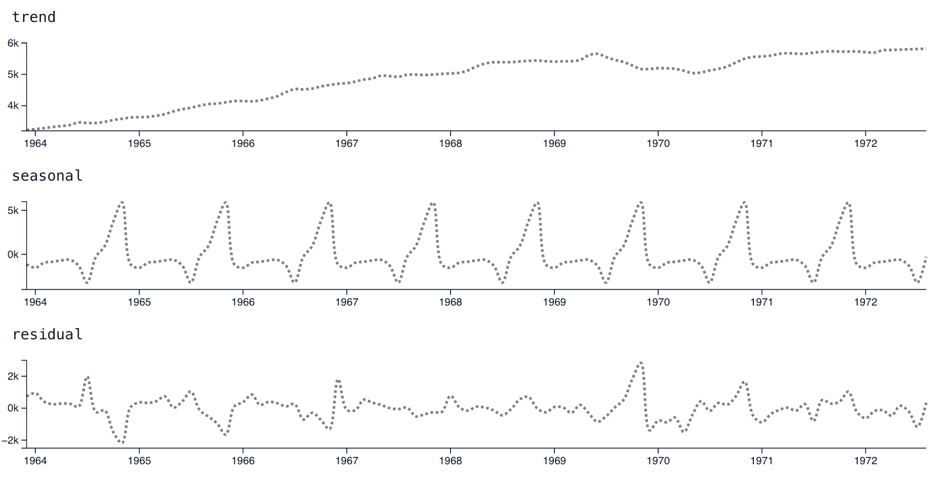
Decomposition
Decomposition is very useful for getting a quick understanding of the main components of most, but not all, time series. Decomposition is a process that takes your selected time series and breaks it down into three components: trend, seasonality, and residual. The three components can be combined with eachother by adding each of the three values at each point in time to get back to the original series.
It is important to note that the three series returned as a result of the decomposition are not neccessarily true or correct. They are simply the best guess given by the algorithm implemented by statsmodels decompose.
- The trend represents long term patterns, often a basic pattern such as overall growth or decline of a market.
- The seasonal component gives insight into repeating patterns in the data. Most business series show a strong weekday seasonality, with spikes or drops on the weekends. Usually an annual seasonality, across winter to summer, also exists. This section allows that pattern to be viewed more closely.
- The residual is everything the trend and seasonal sections cannot account for. A bigger residual is usually a sign of a more-difficult-to-forecast time series, and can sometimes be used to suggest useful regressors if a user is able to discern a pattern to the residuals.
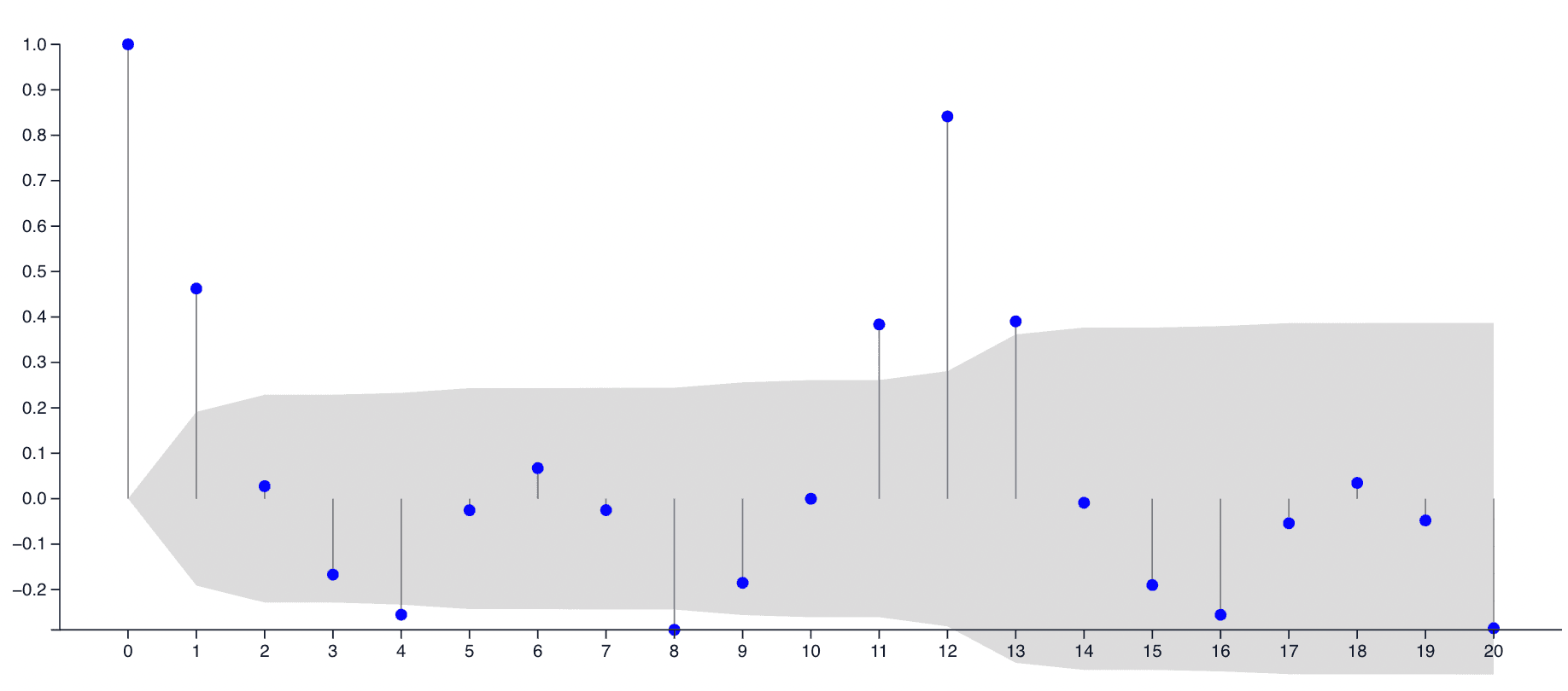
Autocorrelation
Autocorrelation is an analysis of how closely linked a particular time is to a previous record, a lag, in the past. Autocorrelations can reveal hidden patterns in time series. They are also useful for understanding and anticipating outcomes. If a user notices a strong positive autocorrelation with 7 days previously, they know that generally they can anticipate how a series will perform by looking at what happened 7 days previously. This is the basis of autoregressive models like ARIMA. Unfortunately, most real world data does not strictly obey a single lag autocorrelation.
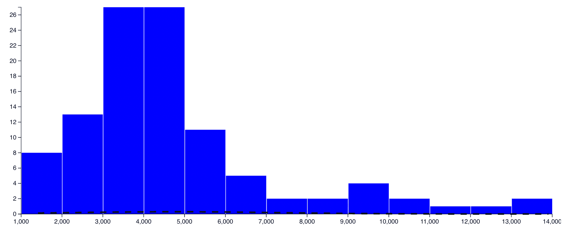
Data Distribution
The distribution of a data is a histogram. There is no right or wrong distribution of the data. Some models will prefer data that is shaped more like a standard normal distribution, with the most data clustered as a hill in the center of the plot, but it is not an absolute requirement. Mostly a distribution is useful for catching potential errors in the data. If an unusually large grouping of very large or very small values is present, these are often worth further inspection.